Công nghệ GSM tổng hợp(xem hiểu liền)hihihihi

TỔNG QUAN VỀ MẠNG DI ĐỘNG GSM

1.GIỚI THIỆU VỀ MẠNG DI ĐỘNG GSM
• Định nghĩa GSM
GSM(Global System of Mobile Communication): mạng thông tin di động toàn cầu-GSM là tiêu chuẩn chung cho các thuê bao di động di chuyển giữa các vị trí địa lý mà vẫn giữ được liên lạc
• Các mạng GSM ở Việt Nam:
Ở Việt Nam và các nước trên thế giới mạng điện thoại GSM vẫn chiếm đa số,Việt Nam có 3 mạng điện thoại GSM đó là:
Vietel : với 5 đầu số 097,098,0166,0168,0169
Vinaphone: với 4 đầu số 091,094,0123,0125
Mobiphone: với 5 đầu số 090,093,0121,0122,0126
• Công nghệ của mạng GSM
Các mạng điện thoại GSM sử dụng công nghệ TDMA(Time Division Multiple Access) : đa truy cập phân chia theo thời giannhằm phân chia thời gian sử dụng mỗi kênh cho nhiều người dùng.
Giải thích: đây là công nghệ cho phép 8 máy di động có thể sử dụng chung 1 kênh để đàm thoại nghĩa là lần lượt từng máy thu phát sau đó ngưng lại để các máy khác thu phát,mỗi máy sẻ sử dụng 1/8 khe thời gian(TS=1 kênh) để truyền và nhận thông tin.
• Công nghệ CDMA
Khác với công nghệ TDMA của các mạng GSM là công nghệ CDMA(Code Division Multiple Access : đa truy cập phân chia theo mã) của các mạng như:
Vietnamobile( tên mới là HT mobile) : sử dụng đầu số 092
Sphone : sử dụng đầu số 095
EVN.Telecom(điện lực) : sử dụng đầu số 0962,0963,0968
Beeline : sử dụng đầu số 0199
Giải thích: công nghệ CDMA sử dụng mã số cho mỗi cuộc gọi và nó không sử dụng một kênh để đàm thoại như công nghệ TDMA mà nó sử dụng cả một phổ tần(nhiều kênh cùng lúc) vì vậy công nghệ này có tốc độ truyền dẫn tín hiệu cao hơn công nghệ TDMA(đa truy cập phân chia theo thời gian).
• Cấu trúc cơ bản của mạng di động
Mỗi mạng điện thoại di động có nhiều tổng đài di động MSC(Mobile Service Switching Center) ở các khu vực khác nhau(ví dụ như tổng đài miền Bắc,tổng đài miền Trung,tổng đài miền Nam) và mỗi tổng đài có nhiều trạm thu phát vô tuyến gốc BTS(Base Transceiver Station)



Chú thích:
MS ( Mobile Station) : máy di động
BTS ( Base Transceiver Station) : trạm thu phát gốc
BSC (Base Station Controller) : bộ điều khiển trạm gốc
MSC (Mobile Service Switching Center) : tổng đài di động( trung tâm chuyển mạch di động)
BSS ( Base Station Subsystem) : phân hệ trạm gốc
PSTN ( Public Switch Telephone Network) : mạng điện thoại chuyển mạch công cộng
PLMN (Public Land Mobile Network ) : mạng di động mặt đất công cộng
ISDN (Integrated Service Digital Network) : mạng số đa dịch vụ
PSPDN(Packet Switch Public Digital Network) : mạng số công cộng chuyển mạch gói
CSPDN (Channel Switch Public Digital Network) : mạng số công cộng chuyển mạch kênh





















NMS (Network Management Subsystem) : phân hệ quản lý mạng
MS ( Mobile Station) : máy di động
-BSS ( Base Station Subsystem) : phân hệ trạm gốc
+BTS(Base Transceiver Station) : trạm thu phát gốc
+ BSC( Base Station Controller ) : bộ điều khiển trạm gốc
+TRAU(Transcoder Rate Adaptor Unit) : đơn vị thích ứng tốc độ và chuyển mã
-SS ( Switching Subsystem) : phân hệ chuyển mạch
+MSC (Mobile Service Switching Center) : tổng đài di động
+VLR (Visitor Location Register) : bộ ghi định vị tạm trú
+HLR (Home Location Register) : bộ ghi định vị thường trú
+GMSC (Gate Mobile Service Switching Center) : tổng đài di động cổng
+AUC (Authentication Center) : trung tâm nhận thực
+EIR (Equipment Identification Register) : bộ ghi nhận dạng thiết bị

PSTN ( Public Switch Telephone Network) : mạng điện thoại chuyển mạch công cộng
PLMN (Public Land Mobile Network ) : mạng di động mặt đất công cộng
ISDN (Integrated Service Digital Network) : mạng số đa dịch vụ
PSPDN(Packet Switch Public Digital Network) : mạng số công cộng chuyển mạch gói
CSPDN (Channel Switch Public Digital Network) : mạng số công cộng chuyển mạch kênh
• Băng tần của GSM 900Mhz
-Nếu bạn đang sử dụng thuê bao di động mạng Vietel(097,098,0166,0168,0169),Vinaphone(091,094,0123,0125),Mobilephone(090,093,0121,0122,0126) là bạn đang sử dụng công nghệ GSM
Công nghệ GSM được chia làm 3 băng tần:
-Băng tần GSM 900Mhz
-Băng tần GSM 1800Mhz
-Băng tần GSM 1900Mhz
-Tất cả các mạng điện thoại GSM ở Việt Nam(Vietel,Vinaphone,Mobilephone) hiện đang sử dụng ở băng tần 900Mhz và 1800Mhz,các nước trên thế giới sử dụng băng tần 900Mhz,Mỹ sử dụng băng tần 1900Mhz
-Tất cả các mạng điện thoại CDMA(Vietnamobile,EVN-Telecom,Sphone,Beeline) ở Việt Nam hiện nay sử dụng băng tần ở 800Mhz




-Với băng tần GSM 900Mhz : Điện thoại di động thu tín hiệu ở dải sóng 935960Mhz và phát tín hiệu ở dải sóng 890915Mhz
- Khoảng cách đường lên(MS phát-BTS thu) và đường xuống(BTS phát-MS thu) của băng GSM 900Mhz luôn là 45Mhz
-Độ rộng mỗi kênh trong GSM 900Mhz là 200Khz=0.2Mhz
-Khi MS thu tín hiệu từ đài phát(BTS) trên một tần số nào đó(nằm trong dãi 935960Mhz) thì nó sẻ trừ đi 45Mhz để lấy ra tần số phát.
• Băng tần GSM 1800Mhz




-Với băng tần 1800Mhz,điện thoại thu tín hiệu(BTS phát-MS thu) ở dải sóng 18051880Mhz và phát tín hiệu(MS phát-BTS thu) ở dải sóng 17101785Mhz
-Khoảng cách đường lên(MS phát-BTS thu) và đường xuống(BTS phát-MS thu) của băng tần GSM 1800 là 95Mhz
-Độ rộng kênh là 200Khz=0.2Mhz
-Khi MS thu tín hiệu từ đài phát(BTS) trên một tần số nào đó (nằm trong dải 18051880Mhz ) thì nó sẻ trừ đi 95Mhz để lấy ra tần số phát.
Nhận xét:
-Băng tần GSM 900Mhz và GSM 1800Mhz thực chất là giống nhau
-
Đặc trưng GSM 900Mhz GSM 1800Mhz
-Băng tần 890960Mhz 17101880Mhz
-Số kênh tần 124 kênh 374 kênh
-Độ rộng kênh 200 Khz 200 Khz
-Phương thức truy cập TDMA TDMA
-Công suất phát 0.8 / 2 / 5W 0,25 / 1 W

• Tái sử dụng tần số trong GSM
-Vì sao phải tái sử dụng tần số?
• Bởi vì tài nguyên tấn số cho mạng di động là rất giới hạn
• Các thuê bao khác nhau phải sử dụng cùng một tần số tại các vị trí khác nhau
• Tuy nhiên chất lượng của đường truyền phải được đảm bảo

-Toàn bộ dải tần phát(MS phát- BTS thu) cho mạng GSM 900Mhz chỉ có từ 890915Mhz tức là : 915-890=25Mhz,độ rộng của mỗi 1 kênh chiếm một khe tần số là 200Khz=0,2Mhz Như vậy toàn bộ dải tần phát 25Mhz của công nghệ GSM 900Mhz sẻ có 125 kênh thoại có thể sử dụng cùng một lúc
-Mỗi kênh thoại(1 byte=8 bit) được chia làm 8 khe thời gian(TS=time slot),trong đó 1/8 khe thời gian dùng cho tín hiệu điều khiển,7/8 khe thời gian còn lại dành cho 7 thuê baonhư vậy tổng số thuê bao có thể liên lạc trong một thời điểm là : 125 kênh x 7 = 875 thuê bao



-875 thuê bao có thể liên lạc trong một thời điểm cho một mạng di độngđây là con số quá ít không đáp ứng được nhu cầu sử dụng của con người,vì vậy tái sử dụng tần số là phương pháp để làm tăng số thuê bao di động có thể liên lạc trong một thời điểm lên tới con số hàng triệu.
Các phương pháp tái sử dụng tần số
-Người ta chia một thành phố ra thành nhiều ô hình lục giác gọi là Cellular(Cell),mỗi Cell được đặt một trạm BTS để thu phát tín hiệu,các Cell không liền kề có thể phát chung một tấn số(như hình dưới thì các ô màu xanh,vàng,đà có thể phát chung tần số)


-Với phương pháp trên người ta có thể chia toàn bộ dải tần(25Mhz=125 kênh=875 thuê bao) ra làm 3 để phát trên các ô không liền kề như 3 màu trên,và như vậy mỗi ô(Cell) có thể phục cho 875/3 = khoảng 291 thuê bao
-Trong một thành phố có thể có hàng trăm trạm thu phát sóng BTS vì vậy nó có thể phục vụ được hàng chục ngàn thuê bao có thể liên lạc trong cùng một thời điểm.
• Phát tín hiệu trong mỗi Cell
Tín hiệu trong mỗi Cell được phát theo một trong hai phương pháp:
-Phát đẳng hướng
-Phát có hướng theo góc 1200(Cell dải quạt 120o)


Cell đẳng hướng và Cell dải quạt 1200
2.CÁC THÀNH PHẦN CỦA MẠNG DI ĐỘNG GSM

Chú thích:
- PSTN ( Public Switch Telephone Network) : mạng điện thoại chuyển mạch công cộng
- MSC (Mobile Service Switching Center) : tổng đài di động( trung tâm chuyển mạch di động)
- BSC (Base Station Controller) : bộ điều khiển trạm gốc
- BTS ( Base Transceiver Station) : trạm thu phát gốc(trạm thu phát vô tuyến)
- MS ( Mobile Station) : máy di động
- : Đường truyền vô tuyến được thực hiện giữa MS với trạm BTS
- : Đường truyền hữu tuyến

• Máy cầm tay di động MS
Trong mỗi máy di động cầm tay khi thực hiện liên lạc,nhà quản lý điều hành mạng sẽ quản lý theo hai mã số.
- Số SIM(Subscriber Identity Module) là mã nhận dạng thuê bao di động dựa vào mã số này mà nhà quản lý có thể quản lý được các cuộc gọi cũng như các dịch vụ gia tăng khác.
- Số IMEI (International Mobile Equipment Identity) là số nhận dạng thiết bị di động quốc tế,số này được nạp vào bộ nhớ ROM của điện thoại khi điện thoại được xuất xưởng,mỗi máy điện thoại có một số IMEI duy nhất.Số IMEI được sử dụng trong mạng GSM để nhận dạng sự hợp pháp của máy đầu cuối(MS).
- Với các công nghệ tiên tiến ngày nay,nếu bạn bật máy điện thoại lên người ta có thể biết bạn đang đứng ở đâu chính xác tới phạm vi 10m2 đó là công nghệ định vị toàn cầu.
-Số IMEI làm được gì?
Các mạng di động ở nước ngoài thường có một thiết bị gọi là EIR( Equipment Identification Register : bộ ghi nhận dạng thiết bị).EIR cho phép kiểm soát và có thể khống chế các ĐTDĐ với số IMEI nằm trong một danh sách cho trước(gọi là danh sách đen-blacklist).Điều này rất hữu ích nếu bạn bị mất máy,bạn chỉ cần thông báo với nhà cung cấp dịch vụ mạng và ĐTDĐ bị mất sẻ không thể sử dụng trong mạng đó nữa.Ở Việt Nam chúng ta do chưa có thiết bị EIR nên chưa có cách nào hữu hiệu để khống chế các máy bị mất cắp hoặc các máy không hợp pháp.
-Cách xem số IMEI trên điện thoại
Vì đây là số nhận thiết bị di động quốc tế nên tất cả các loại máy di động đều sử dụng chung một code để xem
+Cách 1: Bạn bấm *#06#
+Cách 2: Mở nắp Pin,trong thân máy sẻ in dòng IMEI : [ số ]
• Ý nghĩa số IMEI

TAC (Type Approval Code) được kiểm soát bởi trung tâm kiểm soát thiết bị quốc tế
FAC (Final Assembly Code).Do nhà sản xuất ấn định
SNR (Serial Number) : Số SN của máy
SP : Spare-không sử dụng

• Cách để kiểm tra tính hợp lệ của số IMEI
Thuật toán để tính toán số này như sau:
Bước 1: Nhân đôi giá trị của những số ở vị trí lẻ(là các số ở vị trí 1,3,5....,13),trong đó số thứ 1 là số ngoài cùng phía bên phải của chuổi số IMEI
Bước 2: Cộng dồn tất cả các chữ số riêng lẻ của các số thu được ở bước 1,cùng với các số ở vị trí chẵn(là các số ở vị trí 2,4,6…14) trong chuổi số IMEI
Bước 3: Nếu kết quả ở bước 2 là một số chia hết cho 10 thì số A sẽ bằng 0.Còn nếu kết quả ở bước 2 không chia hết cho 10 thì A sẻ bằng số chia hết cho 10 lớn hơn gần nhất trừ đi chính kết quả đó.
Ví dụ : số IMEI là 538008-01-910523-A,trong đó A là số kiểm tra cần phải tính toán.
Bước 1 : 10,16,0,0,18,0,4
Bước 2 : ( 1+0+1+6+0+0+1+8+0+4)+(3+0+8+1+1+5+3)=42
Bước 3 : A = 50-42=8
Như vậy số IMEI hợp lệ phải là : 538008-01-910523-8
• Ý nghĩa số SIM
-SIM(Subcriber Identity Module) là một thẻ thông minh nhỏ gọn chứa cả chương trình và thông tin.
-Các SIM có thể được sử dùng để lưu trữ thông tin của người dùng được định nghĩa như mục danh bạ.
-Một trong những thuận lợi của kiến trúc GSM là SIM có thể di chuyển từ một MS sang MS khác.Điều này làm cho việc nâng cấp rất đơn giản cho người sử dụng điện thoại GSM.







Một IMSI là gì ?
IMSI(International Mobile Subcriber Identity) là một dãy số gồm 15 chữ số được sử dụng để xác định một người sử dụng cá nhân trên mạng GSM
IMSI này bao gồm 3 thành phần:
• MCC(Mobile Coutry Code) :Mã di động quốc gia
• MNC(Mobile Network Code) :Mã mạng di động
• MSIN(Mobile Subsriber Identification Number): Số thuê bao di động

Số thuê bao IMSI

http://didongcdma.vn/forum/archive/index.php/t-2137.html

MCC : Mobile Coutry Code - Mã điện thoại quốc gia,bao gồm 3 số
Ví dụ : Mã điện thoại quốc gia của Việt Nam là “452”
MNC : Mobile Network Code - Mã mạng di động,bao gồm 2 số.
Ví dụ : MNC của Vinaphone là “09”
MSIN : Mobile Subcriber Identification Number- Số thuê bao di động
Ví dụ : 13361818
NMSI : National Mobile Subcriber Identification-Số điện thoại trong nước đầy đủ do MNC và MSIN tạo thành
Ví dụ : 09-13361818
Các giao diện vô tuyến

• Kênh vật lý và kênh logic
-Kênh vật lý là kênh tần số dùng để truyền tải thông tin
Ví dụ : Kênh tần số 890Mhz là kênh vật lý
-Kênh logic là kênh do kênh vật lý chia tách.Trong GSM một kênh vật lý được chia ra làm 8 kênh logic
1 kênh vật lý =8 kênh logic

- Một kênh logic chiếm 1/8 khe thời gian của kênh vật lý
- Kênh vật lý là kênh có tần số xác định,có dải thông là 200Khz
- Thông tin được mang trong một kênh logic được gọi là “Burst” ( cụm)
• Kênh đàm thoại
Lưu lượng các kênh đàm thoại sẽ được truyền đi trên các kênh logic,mỗi kênh vật lý có thể hổ trợ 7 kênh đàm thoại và 1 kênh điều khiển.
• Kênh điều khiển
Mỗi kênh vật lý sử dụng 1/8 khe thời gian làm kênh điều khiển,và 7/8 kênh đàm thoại.Kênh điều khiển sẻ gửi từ đài phát đến máy thu các thông tin điều khiển của tổng đài.

• Điều khiển công suất phát của máy di động
Vì sao phải điều khiển công suất phát của máy di động ?
-Để giảm công suất phát của máy di động khi không cần thiết để tiết kiệm năng lượng tiêu thụ cho pin
-Giảm được nhiễu cho các kênh tần số lân cận
-Giảm ảnh hưởng sức khỏe cho người sử dụng


Ghi chú :
-Công suất phát của máy di động trên xe bus là : 8W
-Công suất phát của máy di động trên xe Taxi là : 5W
-Công suất phát của máy di động bình thường là : 0.8W
• Khi ta bật nguồn Mobile,kênh thu sẻ thu tín hiệu quảng bá của đài phát,tín hiệu thu được đối chiếu với dữ liệu trong bộ nhớ SIM để Mobile có thể nhận ra mạng chủ của mình,sau đó Mobile sẽ phát tín hiệu điều khiển về đài phát(khoảng 34 giây),tín hiệu này được thu qua các trạm BTS và được truyền về tổng đài MSC,tổng đài sẽ ghi lại vị trí của Mobile vào trong Database.
• Sau khi phát tín hiệu về tổng đài,Mobile của bạn sẽ chuyển sang chế độ nghĩ(không phát tín hiệu) và sau khoảng 15 phút nó mới phát tín hiệu điều khiển về tổng đài 1 lần.
• Thu tín hiệu ngắt quảng
- Đài phát phát đi các tín hiệu quảng bá nhưng tín hiệu này cũng phát xen kẽ với các khoảng thời gian rỗi và thời gian phát tin nhắn.


- Khi không có cuộc gọi thì điện thoại sẽ thu được tín hiệu ngắt quảng đủ cho điện thoại giữ được sự liên lạc với tổng đài.
• Khi thuê bao di chuyển giữa các Cell
- Khi bạn đang đứng trong Cell thứ nhất,bạn bật máy và tổng đài thu được tín hiệu trả lời tự động từ điện thoại của bạntổng đài sẽ lưu vị trí của bạn vào trong Database.
-Khi bạn di chuyển sang một Cell khác,nhờ tín hiệu thu được từ kênh quảng bá mà điện thoại của bạn hiểu rằng tín hiệu thu từ trạm BTS thứ nhất đang yếu dần và có một tín hiệu thu từ một trạm BTS khác đang mạnh dần lên.Đến một thời điểm nhất định điện thoại của bạn sẽ tự động phát tín hiệu điều khiển về đài phát để tổng đài ghi lại vị trí mới của bạn
-Khi có một ai đó cầm máy gọi cho bạn,ban đầu nó sẽ phát đi một yêu cầu kết nối đến tổng đài,tổng đài sẽ tìm dấu vết thuê bao của bạn trong cơ sở dữ liệunếu tìm thấy nó sẽ cho kết nối đến trạm BTS mà bạn đang đứng để phát tín hiệu tìm thuê bao của bạn.
-Khi tổng đài nhận được tín hiệu trả lời sẵn sàng kết nối(do máy của bạn phát lại tự động) tổng đài MSC sẽ điều khiển các trạm BTS tìm kênh rỗi để thiết lập cuộc gọilúc này máy của bạn mới có rung và chuông.
3-Các công nghệ vô tuyến

• Các kỹ thuật điều chế tín hiệu
Điều biên - Amplitude Modulation(AM)
Điều tần -Frequency Modulation(FM)
Điều pha-Phase Modulation(PM)
o Kỹ thuật điều(Amplitude Modulation= AM)


Kỹ thuật điều biên làm thay đổi biên độ tín hiệu theo tín hiệu số

o Kỹ thuật điều tần(Frequency Modulation=FM)

Kỹ thuật điều tần làm thay đổi tần số tín hiệu theo tín hiệu số
o Kỹ thuật điều pha (Phase Modulation=PM)





Kỹ thuật điều pha làm thay đổi pha tín hiệu theo tín hiệu số

Công nghệ di động sử dụng kỹ thuật điều pha,đây là kỹ thuật thường được sử dụng cho mạch điều chế số

Chứng chỉ quốc tế .

Các mạch dao động cơ bản

Từ khóa:mạch dao động,khái niệm,thạch anh

1. Mạch tạo dao động

1.1 Mạch dao động hình Sin
Mạch tạo dao động hình Sin từ các linh kiện L – C hoặc từ thạch anh.

* Mạch dao động hình Sin dùng L – C

Mạch dao động hình Sin dùng L – C

• Mach dao động trên có tụ C1 // L1 tạo thành mạch dao động L -C Để duy trì sự dao động này thì tín hiệu dao động được đưa vào chân B của Transistor, R1 là trở định thiên cho Transistor, R2 là trở gánh để lấy ra tín hiệu dao động ra , cuộn dây đấu từ chân E Transistor xuống mass có tác dụng lấy hồi tiếp để duy trì dao động. Tần số dao động của mạch phụ thuộc vào C1 và L1 theo công thức

f = 1 / 2.p.( L1.C1 )1/2

* Mạch dao động hình sin dùng thạch anh

Mạch tạo dao động bằng thạch anh

• X1 : là thạch anh tạo dao động , tần số dao động được ghi trên thân của thach anh, khi thạch anh được cấp điện thì nó tự dao động ra sóng hình sin. Thạch anh thường có tần số dao động từ vài trăm KHz đến vài chục MHz.

• Transistor Q1 khuyếch đại tín hiệu dao động từ thạch anh và cuối cùng tín hiệu được lấy ra ở chân C.

• R1 vừa là điện trở cấp nguồn cho thạch anh vừa định thiên cho transistor Q1

• R2 là trở ghánh tạo ra sụt áp để lấy ra tín hiệu .

1.2. Mạch dao động đa hài

Mạch dao động đa hài tạo xung vuông

* Bạn có thể tự lắp sơ đồ trên với các thông số như sau :

• R1 = R4 = 1 KW

• R2 = R3 = 100KW

• C1 = C2 = 10µF/16V

• Q1 = Q2 = đèn C828

• Hai đèn Led

• Nguồn Vcc là 6V DC

* Giải thích nguyên lý hoạt động

Khi cấp nguồn , giả sử đèn Q1 dẫn trước, áp Uc đèn Q1 giảm => thông qua C1 làm áp Ub đèn Q2 giảm => Q2 tắt => áp Uc đèn Q2 tăng => thông qua C2 làm áp Ub đèn Q1 tăng => xác lập trạng thái Q1 dẫn bão hoà và Q2 tắt , sau khoảng thời gian t , dòng nạp qua R3 vào tụ C1 khi điện áp này > 0,6V thì đèn Q2 dẫn => áp Uc đèn Q2 giảm => tiếp tục như vậy cho đến khi Q2 dẫn bão hoà và Q1 tắt, trạng thái lặp đi lặp lại và tạo thành dao động, chu kỳ dao động phụ thuộc vào C1, C2 và R2, R3.

IC tạo dao động XX555 ; XX có thể là TA hoặc LA v v …

Mạch dao động tạo xung bằng IC 555

• Bạn hãy mua một IC họ 555 và tự lắp cho mình một mạch tạo dao động theo sơ đồ nguyên lý như trên.

• Vcc cung cấp cho IC có thể sử dụng từ 4,5V đến 15V , đường mạch mầu đỏ là dương nguồn, mạch mầu đen dưới cùng là âm nguồn.

• Tụ 103 (10nF) từ chân 5 xuống mass là cố định và bạn có thể bỏ qua ( không lắp cũng được )

• Khi thay đổi các điện trở R1, R2 và giá trị tụ C1 bạn
  sẽ thu được dao động có tần số và độ rộng xung theo ý muốn theo công
  thức.

T = 0.7 × (R1 + 2R2) × C1 và f =	1.4
	(R1 + 2R2) × C1

T = Thời gian của một chu kỳ toàn phần tính bằng (s)
f = Tần số dao động tính bằng (Hz)
R1 = Điện trở tính bằng ohm (W )
R2 = Điện trở tính bằng ohm ( W )
C1 = Tụ điện tính bằng Fara ( W )

T = Tm + Ts
T : chu kỳ toàn phần
Tm = 0,7 x ( R1 + R2 ) x C1 Tm : thời gian điện mức cao
Ts = 0,7 x R2 x C1
Ts : thời gian điện mức thấp

Chu kỳ toàn phần T bao gồm thời gian có điện mức cao Tm và thời gian có điện mức thấp Ts

• Từ các công thức trên ta có thể tạo ra một dao động xung vuông có độ rộng Tm và Ts bất kỳ.

• Sau khi đã tạo ra xung có Tm và Ts ta có T = Tm + Ts và f = 1/ T

* Thí dụ bạn thiết kế mạch tạo xung dùng 555 có Tm = 0,1s , Ts = 1s

Với trị số linh kiện

• C1 = 10µF = 10 x 10-6 = 10-5 F

• R1 = R2 = 100K = 100 x 103 ohm

Tính Ts và Tm = ? Tính tần số f = ?

• Ta có Ts = 0,7 x R2 x C1 = 0,7 x 100.103 x 10-5 = 0,7 s
  Tm = 0,7 x ( R1 + R2 ) x C1 = 0,7 x 200.103 x 105 = 1,4 s

• => T = Tm + Ts = 1,4s + 0,7s = 2,1s

• => f =1 / T = 1/2,1 ~ 0,5 Hz

Mạch dao động nghẹt ( Blocking OSC )

Mạh dao động nghẹt có nguyên tắc hoạt động khá đơn giản, mạch
được sử dụng rộng rãi trong các bộ nguồn xung ( switching ), mạch có cấu tạo như sau :

Mạch dao động nghẹt

Mạch dao động nghẹt bao gồm

• Biến áp : Gồm cuộn sơ cấp 1-2 và cuộn hồi tiếp 3-4, cuộn thứ cấp 5-6

• Transistor Q tham gia dao động và đóng vai trò là đèn công xuất ngắt mở tạo ra dòng điện biến thiên qua cuộn sơ cấp.

• Trở định thiên R1 ( là điện trở mồi )

• R2, C2 là điện trở và tụ điện hồi tiếp

Có hai kiểu mắc hồi tiếp là hồi tiếp dương và hồi tiếp âm, ta xét cấu tạo và nguyên tắc hoạt động của từng mạch.

* Mạch dao động nghẹt hồi tiếp âm

• Mạch hồi tiếp âm có cuộn hồi tiếp 3-4 quấn ngược chiều với cuộn sơ cấp 1-2 , và điện trở mồi R1 có trị số nhỏ khoảng 100K , mạch thường được sử dụng trong các bộ nguồn công xuất nhỏ khoảng 20W trở xuống

• Nguyên tắc hoạt động : Khi cấp nguồn, dòng định thiên qua R1 kích cho đèn Q1 dẫn khá mạnh, dòng qua cuộn sơ cấp 1-2 tăng nhanh tạo ra từ trường biến thiên => cảm ứng sang cuộn hồi
  tiếp, chiều âm của cuộn hồi tiếp được đưa về chân B đèn Q thông qua R2, C2 làm điện áp chân B đèn Q giảm < 0v =""> đèn Q lập tức chuyển sang trạng thái ngắt, sau khoảng thời gian t dòng điện qua R1 nạp vào tụ C2 làm áp chân B đèn Q tăng => đèn Q dẫn lặp lại chu kỳ thứ hai => tạo thành dao động .

• Mạch dao động nghẹt hồi tiếp âm có ưu điểm là dao động nhanh, nhưng có nhược điểm dễ bị xốc điện làm hỏng đèn Q do đó mạch thường không sử dụng trong các bộ nguồn công suất lớn.

* Mạch dao động nghẹt hồi tiếp dương

• Mạch dao động nghẹt hồi tiếp dương có cuộn hồi tiếp 3-4 quấn thuận chiều với cuộn sơ cấp 1-2, điện trở mồi R1 có trị số lớn khoảng 470K

• Vì R1 có trị số lớn, lên dòng định thiên qua R1 ban đầu nhỏ => đèn Q dẫn tăng dần => sinh ra từ trường biến thiên cảm ứng lên cuộn hồi tiếp => điện áp hồi tiếp lấy chiều dương hồi tiếp qua R2, C2 làm đèn Q dẫn tăng => và tiếp tục cho đến khi đèn Q dẫn bão hoà, Khi đèn Q dẫn bão hoà, dòng điện qua cuộn 1-2 không đổi => mất điện áp hồi tiếp => áp chân B đèn Q giảm nhanh và đèn Q lập tức chuyển sang trạng thái ngắt, chu kỳ thứ hai lặp lại như trạng thái ban đầu và tạo thành dao động.

• Mạch này có ưu điểm là rất an toàn dao động từ từ không bị xốc điện, và được sử dụng trong các mạch nguồn công xuất lớn như nguồn Ti vi mầu.

Sưu tầm: Lê viết vĩnh

Band-stop filter

A generic ideal band-stop filter, showing both positive and negative angular frequencies

In signal processing, a band-stop filter or band-rejection filter is a filter that passes most frequencies unaltered, but attenuates those in a specific range to very low levels. It is the opposite of a band-pass filter. A notch filter is a band-stop filter with a narrow stopband (high Q factor). Notch filters are used in live sound reproduction (Public Address systems, also known as PA systems) and in instrument amplifier (especially amplifiers or preamplifiers for acoustic instruments such as acoustic guitar, mandolin, bass instrument amplifier, etc.) to reduce or prevent feedback, while having little noticeable effect on the rest of the frequency spectrum. Other names include 'band limit filter', 'T-notch filter', 'band-elimination filter', and 'band-reject filter'.

Typically, the width of the stopband is less than 1 to 2 decades (that is, the highest frequency attenuated is less than 10 to 100 times the lowest frequency attenuated). In the audio band, a notch filter uses high and low frequencies that may be only semitones apart.

Audio example 1: Anti-hum filter

• Low Freq: 59 Hz
• High Freq: 61 Hz

This means that the filter passes all frequencies, except for the range of 59–61 Hz. This would be used to filter out the mains hum from a 60 Hz power line, though its higher harmonics could still be present. The common European version of the filter would have a 49–51 Hz range.

Audio example 2: Anti-presence filter

• Low Freq: 1 kHz
• High Freq: 4 kHz

RF example 1: Non-linearities of power amplifiers For instance, when measuring non-linearities of power amplifiers a very narrow notch filter could be very useful to avoid the carrier so maximum input power of e.g. a spectrum analyser used to detect spurious content will not be exceeded.

Low-pass filter

A low-pass filter is a filter that passes low-frequency signals but attenuates (reduces the amplitude of) signals with frequencies higher than the cutoff frequency. The actual amount of attenuation for each frequency varies from filter to filter. It is sometimes called a high-cut filter, or treble cut filter when used in audio applications. A low-pass filter is the opposite of a high-pass filter, and a band-pass filter is a combination of a low-pass and a high-pass.

The concept of a low-pass filter exists in many different forms, including electronic circuits (like a hiss filter used in audio), digital algorithms for smoothing sets of data, acoustic barriers, blurring of images, and so on. Low-pass filters play the same role in signal processing that moving averages do in some other fields, such as finance; both tools provide a smoother form of a signal which removes the short-term oscillations, leaving only the long-term trend.

Contents [hide] 1 Examples of low-pass filters 1.1 Acoustic 1.2 Electronic 2 Ideal and real filters 3 Continuous-time low-pass filters 3.1 Laplace notation 4 Electronic low-pass filters 4.1 Passive electronic realization 4.2 Active electronic realization 5 Discrete-time realization 5.1 Algorithmic implementation 6 See also 7 References 8 External links

[edit] Examples of low-pass filters

Figure 1: A low-pass electronic filter realized by an RC circuit

Figure 1 shows a low-pass RC filter for voltage signals, discussed in more detail below. Signal V_out contains frequencies from the input signal, with high frequencies attenuated, but with little attenuation below the cutoff frequency of the filter determined by its RC time constant. For current signals, a similar circuit using a resistor and capacitor in parallel works the same way. See current divider.

[edit] Acoustic

A stiff physical barrier tends to reflect higher sound frequencies, and so acts as a low-pass filter for transmitting sound. When music is playing in another room, the low notes are easily heard, while the high notes are attenuated.

[edit] Electronic

Electronic low-pass filters are used to drive subwoofers and other types of loudspeakers, to block high pitches that they can't efficiently broadcast.

Radio transmitters use low-pass filters to block harmonic emissions which might cause interference with other communications.

The tone knob found on many electric guitars is a low-pass filter used to reduce the amount of treble in the sound.

An integrator is another example of a low-pass filter.

DSL splitters use low-pass and high-pass filters to separate DSL and POTS signals sharing the same pair of wires.

Low-pass filters also play a significant role in the sculpting of sound for electronic music as created by analogue synthesisers. See subtractive synthesis.

[edit] Ideal and real filters

The sinc function, the impulse response of an ideal low-pass filter.

An ideal low-pass filter completely eliminates all frequencies above the cutoff frequency while passing those below unchanged: its frequency response is a rectangular function, and is a brick-wall filter. The transition region present in practical filters does not exist in an ideal filter. An ideal low-pass filter can be realized mathematically (theoretically) by multiplying a signal by the rectangular function in the frequency domain or, equivalently, convolution with its impulse response, a sinc function, in the time domain.

However, the ideal filter is impossible to realize without also having signals of infinite extent, and so generally needs to be approximated for real ongoing signals, because the sinc function's support region extends to all past and future times. The filter would therefore need to have infinite delay, or knowledge of the infinite future and past, in order to perform the convolution. It is effectively realizable for pre-recorded digital signals by assuming extensions of zero into the past and future, or more typically by making the signal repetitive and using Fourier analysis.

Real filters for real-time applications approximate the ideal filter by truncating and windowing the infinite impulse response to make a finite impulse response; applying that filter requires delaying the signal for a moderate period of time, allowing the computation to "see" a little bit into the future. This delay is manifested as phase shift. Greater accuracy in approximation requires a longer delay.

An ideal low-pass filter results in ringing artifacts via the Gibbs phenomenon. These can be reduced or worsened by choice of windowing function, and the design and choice of real filters involves understanding and minimizing these artifacts. For example, "simple truncation [of sinc] causes severe ringing artifacts," in signal reconstruction, and to reduce these artifacts one uses window functions "which drop off more smoothly at the edges."^[1]

The Whittaker–Shannon interpolation formula describes how to use a perfect low-pass filter to reconstruct a continuous signal from a sampled digital signal. Real digital-to-analog converters use real filter approximations.

[edit] Continuous-time low-pass filters

The gain-magnitude frequency response of a first-order (one-pole) low-pass filter. Power gain is shown in decibels (i.e., a 3 dB decline reflects an additional half-power attenuation). Angular frequency is shown on a logarithmic scale in units of radians per second.

There are a great many different types of filter circuits, with different responses to changing frequency. The frequency response of a filter is generally represented using a Bode plot, and the filter is characterized by its cutoff frequency and rate of frequency rolloff. In all cases, at the cutoff frequency, the filter attenuates the input power by half or 3 dB. So the order of the filter determines the amount of additional attenuation for frequencies higher than the cutoff frequency.

• A first-order filter, for example, will reduce the signal amplitude by half (so power reduces by 6 dB) every time the frequency doubles (goes up one octave); more precisely, the power rolloff approaches 20 dB per decade in the limit of high frequency. The magnitude Bode plot for a first-order filter looks like a horizontal line below the cutoff frequency, and a diagonal line above the cutoff frequency. There is also a "knee curve" at the boundary between the two, which smoothly transitions between the two straight line regions. If the transfer function of a first-order low-pass filter has a zero as well as a pole, the Bode plot will flatten out again, at some maximum attenuation of high frequencies; such an effect is caused for example by a little bit of the input leaking around the one-pole filter; this one-pole–one-zero filter is still a first-order low-pass. See Pole–zero plot and RC circuit.

• A second-order filter attenuates higher frequencies more steeply. The Bode plot for this type of filter resembles that of a first-order filter, except that it falls off more quickly. For example, a second-order Butterworth filter will reduce the signal amplitude to one fourth its original level every time the frequency doubles (so power decreases by 12 dB per octave, or 40 dB per decade). Other all-pole second-order filters may roll off at different rates initially depending on their Q factor, but approach the same final rate of 12 dB per octave; as with the first-order filters, zeroes in the transfer function can change the high-frequency asymptote. See RLC circuit.

• Third- and higher-order filters are defined similarly. In general, the final rate of power rolloff for an order-n all-pole filter is 6n dB per octave (i.e., 20n dB per decade).

On any Butterworth filter, if one extends the horizontal line to the right and the diagonal line to the upper-left (the asymptotes of the function), they will intersect at exactly the "cutoff frequency". The frequency response at the cutoff frequency in a first-order filter is 3 dB below the horizontal line. The various types of filters – Butterworth filter, Chebyshev filter, Bessel filter, etc. – all have different-looking "knee curves". Many second-order filters are designed to have "peaking" or resonance, causing their frequency response at the cutoff frequency to be above the horizontal line. See electronic filter for other types.

The meanings of 'low' and 'high' – that is, the cutoff frequency – depend on the characteristics of the filter. The term "low-pass filter" merely refers to the shape of the filter's response; a high-pass filter could be built that cuts off at a lower frequency than any low-pass filter – it is their responses that set them apart. Electronic circuits can be devised for any desired frequency range, right up through microwave frequencies (above 1 GHz) and higher.

[edit] Laplace notation

Continuous-time filters can also be described in terms of the Laplace transform of their impulse response in a way that allows all of the characteristics of the filter to be easily analyzed by considering the pattern of poles and zeros of the Laplace transform in the complex plane (in discrete time, one can similarly consider the Z-transform of the impulse response).

For example, a first-order low-pass filter can be described in Laplace notation as

where s is the Laplace transform variable, τ is the filter time constant, and K is the filter passband gain.

[edit] Electronic low-pass filters

[edit] Passive electronic realization

Passive, first order low-pass RC filter

One simple electrical circuit that will serve as a low-pass filter consists of a resistor in series with a load, and a capacitor in parallel with the load. The capacitor exhibits reactance, and blocks low-frequency signals, causing them to go through the load instead. At higher frequencies the reactance drops, and the capacitor effectively functions as a short circuit. The combination of resistance and capacitance gives you the time constant of the filter τ = RC (represented by the Greek letter tau). The break frequency, also called the turnover frequency or cutoff frequency (in hertz), is determined by the time constant:

or equivalently (in radians per second):

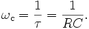
One way to understand this circuit is to focus on the time the capacitor takes to charge. It takes time to charge or discharge the capacitor through that resistor:

• At low frequencies, there is plenty of time for the capacitor to charge up to practically the same voltage as the input voltage.
• At high frequencies, the capacitor only has time to charge up a small amount before the input switches direction. The output goes up and down only a small fraction of the amount the input goes up and down. At double the frequency, there's only time for it to charge up half the amount.

Another way to understand this circuit is with the idea of reactance at a particular frequency:

• Since DC cannot flow through the capacitor, DC input must "flow out" the path marked V_out (analogous to removing the capacitor).
• Since AC flows very well through the capacitor — almost as well as it flows through solid wire — AC input "flows out" through the capacitor, effectively short circuiting to ground (analogous to replacing the capacitor with just a wire).

It should be noted that the capacitor is not an "on/off" object (like the block or pass fluidic explanation above). The capacitor will variably act between these two extremes. It is the Bode plot and frequency response that show this variability.

[edit] Active electronic realization

An active low-pass filter

Another type of electrical circuit is an active low-pass filter.

In the operational amplifier circuit shown in the figure, the cutoff frequency (in hertz) is defined as:

or equivalently (in radians per second):

The gain in the passband is , and the stopband drops off at −6 dB per octave as it is a first-order filter.

Sometimes, a simple gain amplifier (as opposed to the very-high-gain operation amplifier) is turned into a low-pass filter by simply adding a feedback capacitor C. This feedback decreases the frequency response at high frequencies via the Miller effect, and helps to avoid oscillation in the amplifier. For example, an audio amplifier can be made into a low-pass filter with cutoff frequency 100 kHz to reduce gain at frequencies which would otherwise oscillate. Since the audio band (what we can hear) only goes up to 20 kHz or so, the frequencies of interest fall entirely in the passband, and the amplifier behaves the same way as far as audio is concerned.

[edit] Discrete-time realization

For another method of conversion from continuous- to discrete-time, see Bilinear transform.

The effect of a low-pass filter can be simulated on a computer by analyzing its behavior in the time domain, and then discretizing the model.

A simple low-pass RC filter

From the circuit diagram to the right, according to Kirchoff's Laws and the definition of capacitance:

where Q_c(t) is the charge stored in the capacitor at time t. Substituting Equation (Q) into Equation (I) gives , which can be substituted into Equation (V) so that:

This equation can be discretized. For simplicity, assume that samples of the input and output are taken at evenly-spaced points in time separated by Δ_T time. Let the samples of v_in be represented by the sequence , and let v_out be represented by the sequence which correspond to the same points in time. Making these substitutions:

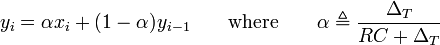
And rearranging terms gives the recurrence relation

That is, this discrete-time implementation of a simple RC low-pass filter is the exponentially-weighted moving average

By definition, the smoothing factor . The expression for α yields the equivalent time constant RC in terms of the sampling period Δ_T and smoothing factor α:

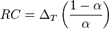
If α = 0.5, then the RC time constant equal to the sampling period. If , then RC is significantly larger than the sampling interval, and .

[edit] Algorithmic implementation

The filter recurrence relation provides a way to determine the output samples in terms of the input samples and the preceding output. The following pseudocode algorithm will simulate the effect of a low-pass filter on a series of digital samples:

 // Return RC low-pass filter output samples, given input samples,
// time interval dt, and time constant RC
function lowpass(real[0..n] x, real dt, real RC)
  var real[0..n] y
  var real α := dt / (RC + dt)
  y[0] := x[0]
  for i from 1 to n
      y[i] := α * x[i] + (1-α) * y[i-1]   
  return y

The loop which calculates each of the n outputs can be refactored into the equivalent:

   for i from 1 to n
      y[i] := y[i-1] + α * (x[i] - y[i-1])

That is, the change from one filter output to the next is proportional to the difference between the previous output and the next input. This exponential smoothing property matches the exponential decay seen in the continuous-time system. As expected, as the time constant RC increases, the discrete-time smoothing parameter α decreases, and the output samples respond more slowly to a change in the input samples – the system will have more inertia.

High-pass filter

A high-pass filter is an LTI filter that passes high frequencies well but attenuates (i.e., reduces the amplitude of) frequencies lower than the cutoff frequency. The actual amount of attenuation for each frequency is a design parameter of the filter. It is sometimes called a low-cut filter; the terms bass-cut filter or rumble filter are also used in audio applications.^{[citation needed]}

Contents [hide] 1 First-order continuous-time implementation 2 Discrete-time realization 2.1 Algorithmic implementation 3 Applications 4 See also 5 References 6 External links

[edit] First-order continuous-time implementation

Figure 1: A passive, analog, first-order high-pass filter, realized by an RC circuit

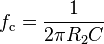
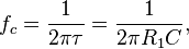
The simple first-order electronic high-pass filter shown in Figure 1 is implemented by placing an input voltage across the series combination of a capacitor and a resistor and using the voltage across the resistor as an output. The product of the resistance and capacitance (R×C) is the time constant (τ); it is inversely proportional to the cutoff frequency f_c, at which the output power is half (−3 dB) the input power. That is,

where f_c is in Hertz, τ is in seconds, R is in Ohms, and C is in Farads.

Figure 2: An active high-pass filter

Figure 2 shows an active electronic implementation of a first-order high-pass filter using an operational amplifier. In this case, the filter has a passband gain of -R₂/R₁ and has a corner frequency of

Because this filter is active, it may have non-unity passband gain. That is, high-frequency signals are inverted and amplified by R₂/R₁.

[edit] Discrete-time realization

For another method of conversion from continuous- to discrete-time, see Bilinear transform.

Discrete-time high-pass filters can also be designed. Discrete-time filter design is beyond the scope of this article; however, a simple example comes from the conversion of the continuous-time high-pass filter above to a discrete-time realization. That is, the continuous-time behavior can be discretized.

From the circuit in Figure 1 above, according to Kirchoff's Laws and the definition of capacitance:

where Q_c(t) is the charge stored in the capacitor at time t. Substituting Equation (Q) into Equation (I) and then Equation (I) into Equation (V) gives:

This equation can be discretized. For simplicity, assume that samples of the input and output are taken at evenly-spaced points in time separated by Δ_T time. Let the samples of V_in be represented by the sequence , and let V_out be represented by the sequence which correspond to the same points in time. Making these substitutions:

And rearranging terms gives the recurrence relation

That is, this discrete-time implementation of a simple continuous-time RC high-pass filter is

By definition, . The expression for parameter α yields the equivalent time constant RC in terms of the sampling period Δ_T and α:

If α = 0.5, then the RC time constant equal to the sampling period. If , then RC is significantly smaller than the sampling interval, and .

[edit] Algorithmic implementation

The filter recurrence relation provides a way to determine the output samples in terms of the input samples and the preceding output. The following pseudocode algorithm will simulate the effect of a high-pass filter on a series of digital samples:

 // Return RC high-pass filter output samples, given input samples,
// time interval dt, and time constant RC
function highpass(real[0..n] x, real dt, real RC)
  var real[0..n] y
  var real α := RC / (RC + dt)
  y[0] := x[0]
  for i from 1 to n
    y[i] := α * y[i-1] + α * (x[i] - x[i-1])
  return y

The loop which calculates each of the n outputs can be refactored into the equivalent:

   for i from 1 to n
    y[i] := α * (y[i-1] + x[i] - x[i-1])

However, the earlier form shows how the parameter α changes the impact of the prior output y[i-1] and current change in input (x[i] - x[i-1]). In particular,

• A large α implies that the output will decay very slowly but will also be strongly influenced by even small changes in input. By the relationship between parameter α and time constant RC above, a large α corresponds to a large RC and therefore a low corner frequency of the filter. Hence, this case corresponds to a high-pass filter with a very narrow stop band. Because it is excited by small changes and tends to hold its prior output values for a long time, it can pass relatively low frequencies. However, a constant input (i.e., an input with (x[i] - x[i-1])=0) will always decay to zero, as would be expected with a high-pass filter with a large RC.
• A small α implies that the output will decay quickly and will require large changes in the input (i.e., (x[i] - x[i-1]) is large) to cause the output to change much. By the relationship between parameter α and time constant RC above, a small α corresponds to a small RC and therefore a high corner frequency of the filter. Hence, this case corresponds to a high-pass filter with a very wide stop band. Because it requires large (i.e., fast) changes and tends to quickly forget its prior output values, it can only pass relatively high frequencies, as would be expected with a high-pass filter with a small RC.

[edit] Applications

Such a filter could be used as part of an audio crossover to direct high frequencies to a tweeter while blocking bass signals which could interfere with, or damage, the speaker. When such a filter is built into a loudspeaker cabinet it is normally a passive filter that also includes a low-pass filter for the woofer and so often employs both a capacitor and inductor (although very simple high-pass filters for tweeters can consist of a series capacitor and nothing else). An alternative, which provides good quality sound without inductors (which are prone to parasitic coupling, are expensive, and may have significant internal resistance) is to employ bi-amplification with active RC filters with separate power amplifiers for each loudspeaker making an active crossover.^{[citation needed]}

Rumble filters are high-pass filters applied to the removal of unwanted sounds below or near to the lower end of the audible range. For example, noises (e.g., footsteps, or motor noises from record players and tape decks) may be removed because they are undesired or may overload the RIAA equalization circuit of the preamp.^{[citation needed]}

High-pass and low-pass filters are also used in digital image processing to perform transformations in the spatial frequency domain.^{[citation needed]}

High-pass filters are also used for AC coupling at the input and output of amplifiers.^{[citation needed]}